4. Functions

4.1. Functions

In Python, a function is a named sequence of statements that belong together. Their primary purpose is to help us organize programs into chunks that match how we think about the problem.

The syntax for a function definition is:

def NAME( PARAMETERS ):
    STATEMENTS

We can make up any names we want for the functions we create, except that we can’t use a name that is a Python keyword, and the names must follow the rules for legal identifiers. By convention, we like to use all lowercase for function names, with words separated by underscores, such as draw_square.

There can be any number of statements inside the function, but they have to be indented from the def. In the examples in this book, we will use the standard indentation of four spaces. Function definitions are the second of several compound statements we will see, all of which have the same pattern:

A header line which begins with a keyword and ends with a colon.
A body consisting of one or more Python statements, each indented the same amount — we strongly recommend 4 spaces — from the header line.

We’ve already seen the for loop which follows this pattern.

So looking again at the function definition, the keyword in the header is def, which is followed by the name of the function and some parameters enclosed in parentheses. The parameter list may be empty, or it may contain any number of parameters separated from one another by commas. In either case, the parentheses are required. The parameters specifies what information, if any, we have to provide in order to use the new function.

Suppose we’re working with turtles, and a common operation we need is to draw squares. “Draw a square” is an abstraction, or a mental chunk, of a number of smaller steps. So let’s write a function to capture the pattern of this “building block”:

import turtle

def draw_square(t, sz):
    """Make turtle t draw a square of sz."""
    for i in range(4):
        t.forward(sz)
        t.left(90)

wn = turtle.Screen()        # Set up the window and its attributes
wn.bgcolor("lightgreen")
wn.title("Alex meets a function")

alex = turtle.Turtle()      # Create alex
draw_square(alex, 50)       # Call the function to draw the square

wn.mainloop()

This function is named draw_square. It has two parameters: one to tell the function which turtle to move around, and the other to tell it the size of the square we want drawn. Make sure you know where the body of the function ends — it depends on the indentation, and the blank lines don’t count for this purpose!

Docstrings for documentation

If the first thing after the function header is a string, it is treated as a docstring and gets special treatment in Python and in some programming tools. For example, when we when we type help('funcname') in the IDLE shell (where “funcname” is the name of the function), we get a message telling us what arguments the function takes, and it shows us any other text contained in the docstring. For example, type help('print') in the IDLE shell and read the message that you get.

Docstrings are the key way to document our functions in Python and the documentation part is important. Because whoever calls our function shouldn’t have to need to know what is going on in the function or how it works; they just need to know what arguments our function takes, what it does, and what the expected result is. Enough to be able to use the function without having to look underneath. This goes back to the concept of abstraction of which we’ll talk more about.

Docstrings are usually formed using triple-quoted strings as they allow us to easily expand the docstring later on should we want to write more than a one-liner.

Just to differentiate from comments, a string at the start of a function (a docstring) is retrievable by Python tools at runtime. By contrast, comments are completely eliminated when the program is parsed.

Defining a new function does not make the function run. To do that we need a function call. We’ve already seen how to call some built-in functions like print, range and int. Function calls contain the name of the function being executed followed by a list of values, called arguments, which are assigned to the parameters in the function definition. So in line 14 of the program above, we call the function, and pass alex as the turtle to be manipulated, and 50 as the size of the square we want. While the function is executing, then, the variable sz refers to the value 50, and the variable t refers to the same turtle instance that the variable alex refers to.

Once we’ve defined a function, we can call it as often as we like, and its statements will be executed each time we call it. And we could use it to get any of our turtles to draw a square. In the next example, we’ve changed the draw_square function a little, and we get tess to draw 15 squares, with some variations.

import turtle

def draw_multicolor_square(t, sz):
    """Make turtle t draw a multi-color square of sz."""
    for i in ["red", "purple", "hotpink", "blue"]:
        t.color(i)
        t.forward(sz)
        t.left(90)

wn = turtle.Screen()        # Set up the window and its attributes
wn.bgcolor("lightgreen")

tess = turtle.Turtle()      # Create tess and set some attributes
tess.pensize(3)

size = 20                   # Size of the smallest square
for i in range(15):
    draw_multicolor_square(tess, size)
    size = size + 10        # Increase the size for next time
    tess.forward(10)        # Move tess along a little
    tess.right(18)          #    and give her some turn

wn.mainloop()

4.2. Functions can call other functions

Let’s assume now we want a function to draw a rectangle. We need to be able to call the function with different arguments for width and height. And, unlike the case of the square, we cannot repeat the same thing 4 times, because the four sides are not equal.

So we eventually come up with this rather nice code that can draw a rectangle.

def draw_rectangle(t, w, h):
    """Get turtle t to draw a rectangle of width w and height h."""
    for i in range(2):
        t.forward(w)
        t.left(90)
        t.forward(h)
        t.left(90)

The parameter names are deliberately chosen as single letters to ensure they’re not misunderstood. In real programs, once we’ve had more experience, we will insist on better variable names than this. But the point is that the program doesn’t “understand” that we’re drawing a rectangle, or that the parameters represent the width and the height. Concepts like rectangle, width, and height are the meaning we humans have, not concepts that the program or the computer understands.

Thinking like a computer scientist involves looking for patterns and relationships. In the code above, we’ve done that to some extent. We did not just draw four sides. Instead, we spotted that we could draw the rectangle as two halves, and used a loop to repeat that pattern twice.

But now we might spot that a square is a special kind of rectangle. We already have a function that draws a rectangle, so we can use that to draw our square.

def draw_square(tx, sz):        # A new version of draw_square
    draw_rectangle(tx, sz, sz)

There are some points worth noting here:

Functions can call other functions.
Rewriting draw_square like this captures the relationship that we’ve spotted between squares and rectangles.
A caller of this function might say draw_square(tess, 50). The parameters of this function, tx and sz, are assigned the values of the tess object, and the int 50 respectively.
In the body of the function they are just like any other variable.
When the call is made to draw_rectangle, the values in variables tx and sz are fetched first, then the call happens. So as we enter the top of function draw_rectangle, its variable t is assigned the tess object, and w and h in that function are both given the value 50.

So far, it may not be clear why it is worth the trouble to create all of these new functions. Actually, there are a lot of reasons, but this example demonstrates two:

Creating a new function gives us an opportunity to name a group of statements. Functions can simplify a program by hiding a complex computation behind a single command. The function (including its name) can capture our mental chunking, or abstraction, of the problem.
Creating a new function can make a program smaller by eliminating repetitive code.

As we might expect, we have to create a function before we can execute it. In other words, the function definition has to be executed before the function is called.

4.3. Flow of execution

In order to ensure that a function is defined before its first use, we have to know the order in which statements are executed, which is called the flow of execution. We’ve already talked about this a little in the previous chapter.

Execution always begins at the first statement of the program. Statements are executed one at a time, in order from top to bottom.

Function definitions do not alter the flow of execution of the program, but remember that statements inside the function are not executed until the function is called. Although it is not common, we can define one function inside another. In this case, the inner definition isn’t executed until the outer function is called.

Function calls are like a detour in the flow of execution. Instead of going to the next statement, the flow jumps to the first line of the called function, executes all the statements there, and then comes back to pick up where it left off.

That sounds simple enough, until we remember that one function can call another. While in the middle of one function, the program might have to execute the statements in another function. But while executing that new function, the program might have to execute yet another function!

Fortunately, Python is adept at keeping track of where it is, so each time a function completes, the program picks up where it left off in the function that called it. When it gets to the end of the program, it terminates.

What’s the moral of this sordid tale? When we read a program, don’t read from top to bottom. Instead, follow the flow of execution.

4.4. Functions that require arguments

Most functions require arguments: the arguments provide for generalization. For example, if we want to find the absolute value of a number, we have to indicate what the number is. Python has a built-in function for computing the absolute value:

>>> abs(5)
5
>>> abs(-5)
5

In this example, the arguments to the abs function are 5 and -5.

Some functions take more than one argument. For example the built-in function pow takes two arguments, the base and the exponent. Inside the function, the values that are passed get assigned to variables called parameters.

>>> pow(2, 3)
8
>>> pow(7, 4)
2401

Another built-in function that takes more than one argument is max.

>>> max(7, 11)
11
>>> max(4, 1, 17, 2, 12)
17
>>> max(3 * 11, 5**3, 512 - 9, 1024**0)
503

max can be passed any number of arguments, separated by commas, and will return the largest value passed. The arguments can be either simple values or expressions. In the last example, 503 is returned, since it is larger than 33, 125, and 1.

4.5. Functions that return values

All the functions in the previous section return values. Furthermore, functions like range, int, abs all return values that can be used to build more complex expressions.

So an important difference between these functions and one like draw_square is that draw_square was not executed because we wanted it to compute a value — on the contrary, we wrote draw_square because we wanted it to execute a sequence of steps that caused the turtle to draw.

A function that returns a value is called a fruitful function in this book. The opposite of a fruitful function is void function — one that is not executed for its resulting value, but is executed because it does something useful. (Languages like Java, C#, C and C++ use the term “void function”, other languages like Pascal call it a procedure.) Even though void functions are not executed for their resulting value, Python always wants to return something. So if the programmer doesn’t arrange to return a value, Python will automatically return the value None.

How do we write our own fruitful function? Below is the standard formula for compound interest, which we’ll now write as a fruitful function:

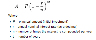
def final_amt(p, r, n, t):
    """
    Apply the compound interest formula to p
    to produce the final amount.
    """
    a = p * (1 + r/n) ** (n*t)
    return a         # This is new, and makes the function fruitful.

# now that we have the function above, let us call it.
toInvest = float(input("How much do you want to invest?"))
fnl = final_amt(toInvest, 0.08, 12, 5)
print("At the end of the period you will have " + str(fnl))

The return statement is followed an expression (a in this case). This expression will be evaluated and returned to the caller as the “fruit” of calling this function.
We prompted the user for the principal amount. The type of toInvest is a string, but we need a number before we can work with it. Because it is money, and could have decimal places, we’ve used the float type converter function to parse the string and return a float.
Notice how we entered the arguments for 8% interest, compounded 12 times per year, for 5 years.
When we run this, if you use 10000 as your input, you’ll get the output

At the end of the period you’ll have 14898.457083

This is a bit messy with all these decimal places, but remember that Python doesn’t understand that we’re working with money: it just does the calculation to the best of its ability, without rounding.
The line toInvest = float(input("How much do you want to invest?")) also shows yet another example of composition — we can call a function like float, and its arguments can be the results of other function calls (like input) that we’ve called along the way.

Notice something else very important here. The name of the variable we pass as an argument — toInvest — has nothing to do with the name of the parameter — p. It is as if p = toInvest is executed when final_amt is called. It doesn’t matter what the value was named in the caller, in final_amt its name is p.

These short variable names are getting quite tricky, so perhaps we’d prefer one of these versions instead:

def final_amt_v2(principalAmount, nominalPercentageRate,
                     numTimesPerYear, years):
    a = principalAmount * (1 + nominalPercentageRate /
              numTimesPerYear) ** (numTimesPerYear*years)
    return a

def final_amt_v3(amt, rate, compounded, years):
    a = amt * (1 + rate/compounded) ** (componded*years)
    return a

They all do the same thing. Use your judgement to write code that can be best understood by other humans! Short variable names are more economical and sometimes make code easier to read: E = mc² would not be nearly so memorable if Einstein had used longer variable names! If you do prefer short names, make sure you also have some comments to enlighten the reader about what the variables are used for.

4.6. Variables and parameters are local

When we create a local variable inside a function, it only exists inside the function, and we cannot use it outside. For example, consider again this function:

def final_amt(p, r, n, t):
    a = p * (1 + r/n) ** (n*t)
    return a

If we try to use a, outside the function, we’ll get an error:

Traceback (most recent call last):
      File "<pyshell#12>", line 1, in <module>
        a
NameError: name 'a' is not defined

The variable a is local to final_amt, and is not visible outside the function.

Additionally, a only exists while the function is being executed — we call this its lifetime. When the execution of the function terminates, the local variables are destroyed.

Parameters are also local, and act like local variables. For example, the lifetimes of p, r, n, t begin when final_amt is called, and the lifetime ends when the function completes its execution.

So it is not possible for a function to set some local variable to a value, complete its execution, and then when it is called again next time, recover the local variable. Each call of the function creates new local variables, and their lifetimes expire when the function returns to the caller.

4.7. Turtles Revisited

Now that we have fruitful functions, we can focus our attention on reorganizing our code so that it fits more nicely into our mental chunks. This process of rearrangement is called refactoring the code.

Two things we’re always going to want to do when working with turtles is to create the window for the turtle, and to create one or more turtles. For example, we could write some functions to make these tasks easier in future:

def make_window(colr, ttle):
    """
     Set up the window with the given background color and title.
     Returns the new window.
    """
    w = turtle.Screen()
    w.bgcolor(colr)
    w.title(ttle)
    return w


def make_turtle(colr, sz):
    """
     Set up a turtle with the given color and pensize.
     Returns the new turtle.
    """
    t = turtle.Turtle()
    t.color(colr)
    t.pensize(sz)
    return t

Then we could make new turtles easily, like so:

wn = make_window("lightgreen", "Tess and Alex dancing")
tess = make_turtle("hotpink", 5)
alex = make_turtle("black", 1)
dave = make_turtle("yellow", 2)

The trick about refactoring code is to anticipate which things we are likely to want to change each time we call the function: these should become the parameters, or changeable parts, of the functions we write.

4.8. Return values

The built-in functions we have used, such as abs, pow, int, max, and range, have produced results. Calling each of these functions generates a value, which we usually assign to a variable or use as part of an expression.

biggest = max(3, 7, 2, 5)
x = abs(3 - 11) + 10

We also wrote our own function to return the final amount for a compound interest calculation.

We are going to write more functions that return values, which we will call fruitful functions, for want of a better name. The first example is area, which returns the area of a circle with the given radius:

def area(radius):
    b = 3.14159 * radius**2
    return b

We have seen the return statement before: in a fruitful function the return statement includes a return value. This statement means: evaluate the return expression, and then return it immediately as the result (the fruit) of this function. The expression provided can be arbitrarily complicated, so we could have written this function like this:

def area(radius):
    return 3.14159 * radius * radius

On the other hand, temporary variables like b above often make debugging easier.

4.9. Program development

At this point, you should be able to look at complete functions and tell what they do. Also, you have already written some small functions. As you write larger functions, you might start to have more difficulty, especially with runtime and semantic errors.

To deal with increasingly complex programs, we are going to suggest a technique called incremental development. The goal of incremental development is to avoid long debugging sessions by adding and testing only a small amount of code at a time.

As an example, suppose we want to find the distance between two points, given by the coordinates (x₁, y₁) and (x₂, y₂). By the Pythagorean theorem, the distance is:

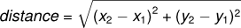
Don’t worry if you don’t know this formula or how to prove it. We’re just going to worry about how to implement it in Python.

The first step is to consider what a distance function should look like in Python. In other words, what are the inputs (parameters) and what is the output (return value)?

In this case, the two points are the inputs, which we can represent using four parameters. The return value is the distance, which is a floating-point value.

Already we can write an outline of the function that captures our thinking so far:

def distance(x1, y1, x2, y2):
   return 0.0

Obviously, this version of the function doesn’t compute distances; it always returns zero. But it is syntactically correct, and it will run, which means that we can test it before we make it more complicated.

To test the new function, we call it with sample values:

def distance(x1, y1, x2, y2):
    return 0.0

print(distance(1,2,4,6))

We chose these values so that the horizontal distance equals 3 and the vertical distance equals 4; that way, the result is 5 (the hypotenuse of a 3-4-5 triangle). When testing a function, it is useful to know the right answer.

At this point we have confirmed that the function is syntactically correct, and we can start adding lines of code. After each incremental change, we test the function again. If an error occurs at any point, we know where it must be — in the last line we added.

A logical first step in the computation is to find the differences x₂- x₁ and y₂- y₁. We will refer to those values using temporary variables named dx and dy.

def distance(x1, y1, x2, y2):
    dx = x2 - x1
    dy = y2 - y1
    return 0.0

print(distance(1,2,4,6))

If we call the function with the arguments shown above, when the flow of execution gets to the return statement, dx should be 3 and dy should be 4. We can check that this is the case by putting in temporary print statements in the function, like so:

def distance(x1, y1, x2, y2):
    dx = x2 - x1
    dy = y2 - y1
    print("dx = "+str(dx))
    print("dy = "+str(dy))
    return 0.0

print(distance(1,2,4,6))

Now we can confirm that the function is getting the right parameters and performing the first computation correctly. If not, there are only a few lines to check. Once we’re sure that dx and dy are working correctly, we should remove the temporary print statements — we don’t want them in our final program.

Next we compute the sum of squares of dx and dy:

def distance(x1, y1, x2, y2):
    dx = x2 - x1
    dy = y2 - y1
    dsquared = dx*dx + dy*dy
    return 0.0

print(distance(1,2,4,6))

Again, we could put in a temporary print statement, then run the program at this stage and check the value of dsquared (which should be 25):

def distance(x1, y1, x2, y2):
    dx = x2 - x1
    dy = y2 - y1
    dsquared = dx*dx + dy*dy
    print("dsquared = "+str(dsquared))
    return 0.0

print(distance(1,2,4,6))

Finally, using the fractional exponent 0.5 to find the square root, we compute and return the result:

def distance(x1, y1, x2, y2):
    dx = x2 - x1
    dy = y2 - y1
    dsquared = dx*dx + dy*dy
    result = dsquared**0.5
    return result

print(distance(1,2,4,6))

If that works correctly, you are done. Otherwise, you might want to inspect the value of result before the return statement.

When you start out, you might add only a line or two of code at a time. As you gain more experience, you might find yourself writing and debugging bigger conceptual chunks. Either way, stepping through your code one line at a time and verifying that each step matches your expectations can save you a lot of debugging time. As you improve your programming skills you should find yourself managing bigger and bigger chunks: this is very similar to the way we learned to read letters, syllables, words, phrases, sentences, paragraphs, etc., or the way we learn to chunk music — from individual notes to chords, bars, phrases, and so on.

The key aspects of the process are:

Start with a working skeleton program and make small incremental changes. At any point, if there is an error, you will know exactly where it is.
Use temporary variables to refer to intermediate values so that you can easily inspect and check them.
Once the program is working, relax, sit back, and play around with your options. (There is interesting research that links “playfulness” to better understanding, better learning, more enjoyment, and a more positive mindset about what you can achieve — so spend some time fiddling around!) You might want to consolidate multiple statements into one bigger compound expression, or rename the variables you’ve used, or see if you can make the function shorter. A good guideline is to aim for making code as easy as possible for others to read.

Here is another version of the function. It makes use of a square root function that is in the math module. Which do you prefer? Which looks “closer” to the Pythagorean formula we started out with?

import math

def distance(x1, y1, x2, y2):
    return math.sqrt((x2-x1)**2 + (y2-y1)**2)

print(distance(1,2,4,6))

As we saw in the example above, a powerful technique for debugging is to insert extra print functions in carefully selected places in your code. Then, by inspecting the output of the program, you can check whether the algorithm is doing what you expect it to. Be clear about the following, however:

You must have a clear solution to the problem, and must know what should happen before you can debug a program. Work on solving the problem on a piece of paper (perhaps using a flowchart to record the steps you take) before you concern yourself with writing code. Writing a program doesn’t solve the problem — it simply automates the manual steps you would take. So first make sure you have a pen-and-paper manual solution that works. Programming then is about making those manual steps happen automatically.
Do not write chatterbox functions. A chatterbox is a fruitful function that, in addition to its primary task, also asks the user for input, or prints output, when it would be more useful if it simply shut up and did its work quietly.

For example, we’ve seen built-in functions like range, max and abs. None of these would be useful building blocks for other programs if they prompted the user for input, or printed their results while they performed their tasks.

So a good tip is to avoid calling print and input functions inside fruitful functions, unless the primary purpose of your function is to perform input and output. The exception to this rule is to temporarily sprinkle some calls to print into your code to help debug and understand what is happening when the code runs, but these will then be removed once you get things working.

4.10. Glossary

argument

A value provided to a function when the function is called. This value is assigned to the corresponding parameter in the function. The argument can be the result of an expression which may involve operators, operands and calls to other fruitful functions.

body

The second part of a compound statement. The body consists of a sequence of statements all indented the same amount from the beginning of the header. The standard amount of indentation used within the Python community is 4 spaces.

chatterbox function

A function which interacts with the user (using input or print) when it should not. Silent functions that just convert their input arguments into their output results are usually the most useful ones.

composition (of functions)

Calling one function from within the body of another, or using the return value of one function as an argument to the call of another.

compound statement

A statement that consists of two parts:

header - which begins with a keyword determining the statement type, and ends with a colon.
body - containing one or more statements indented the same amount from the header.

The syntax of a compound statement looks like this:

keyword ... :
    statement
    statement ...

dead code

Part of a program that can never be executed, often because it appears after a return statement.

docstring

A special string that is attached to a function as its __doc__ attribute. Tools like IDLE can use docstrings to provide documentation or hints for the programmer. When we get to modules, classes, and methods, we’ll see that docstrings can also be used there.

flow of execution

The order in which statements are executed during a program run.

fruitful function

A function that yields a return value instead of None.

function

A named sequence of statements that performs some useful operation. Functions may or may not take parameters and may or may not produce a result.

function call

A statement that executes a function. It consists of the name of the function followed by a list of arguments enclosed in parentheses.

function composition

Using the output from one function call as the input to another.

function definition

A statement that creates a new function, specifying its name, parameters, and the statements it executes.

fruitful function

A function that returns a value when it is called.

header line

The first part of a compound statement. A header line begins with a keyword and ends with a colon (:)

import statement

A statement which permits functions and variables defined in another Python module to be brought into the environment of another script. To use the features of the turtle, we need to first import the turtle module.

incremental development

A program development plan intended to simplify debugging by adding and testing only a small amount of code at a time.

lifetime

Variables and objects have lifetimes — they are created at some point during program execution, and will be destroyed at some time.

local variable

A variable defined inside a function. A local variable can only be used inside its function. Parameters of a function are also a special kind of local variable.

None

A special Python value. One use in Python is that it is returned by functions that do not execute a return statement with a return argument.

parameter

A name used inside a function to refer to the value which was passed to it as an argument.

refactor

A fancy word to describe reorganizing our program code, usually to make it more understandable. Typically, we have a program that is already working, then we go back to “tidy it up”. It often involves choosing better variable names, or spotting repeated patterns and moving that code into a function.

return value

The value provided as the result of a function call.

scaffolding

Code that is used during program development to assist with development and debugging. The unit test code that we added in this chapter are examples of scaffolding.

temporary variable

A variable used to store an intermediate value in a complex calculation.

test suite

A collection of tests for some code you have written.

traceback

A list of the functions that are executing, printed when a runtime error occurs. A traceback is also commonly refered to as a stack trace, since it lists the functions in the order in which they are stored in the runtime stack.

unit testing

An automatic procedure used to validate that individual units of code are working properly. Having a test suite is extremely useful when somebody modifies or extends the code: it provides a safety net against going backwards by putting new bugs into previously working code. The term regression testing is often used to capture this idea that we don’t want to go backwards!

void function

The opposite of a fruitful function: one that does not return a value. It is executed for the work it does, rather than for the value it returns.

Navigation